Deep Learning has been massively successful in recent years, in part because of the efficiency of its learning algorithm: backpropagation. However, the brain is also pretty good at learning(citation needed), and it’s definitely not doing backprop. One theory for how the brain learns, is Predictive Coding (PC), which has recently been repurposed as a biologically-plausible alternative to backpropagation.
Coming from theoretical neuroscience, PC is often described in overly complicated and confusing ways, with free energies and variational inference. While technically correct, it’s not very helpful to gain intuition on how PC works, and it might scare off newcomers looking for entry into the field.
So, to maintain my sanity, I developed an interpretation of PC that better fit my Deep Learning background: Predictive Coding is just backpropagation with local losses.
Let me explain.
Predictive Coding: inserting local losses into the network
Consider the following feedforward architecture:
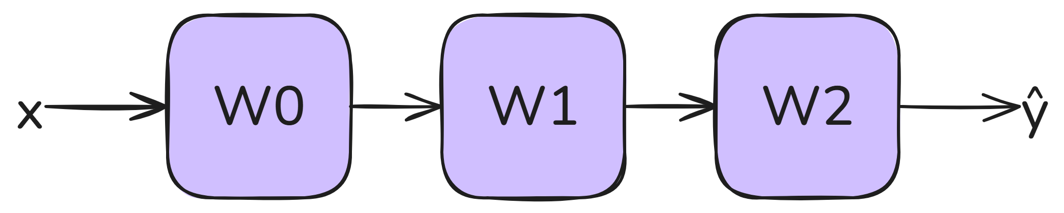
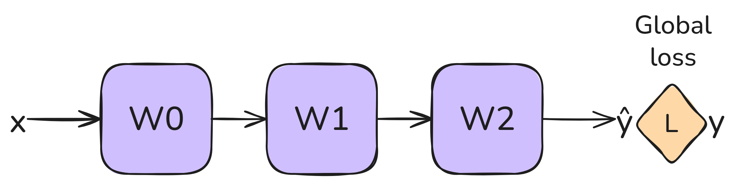
Typically, with backprop, we’d train this with a single global loss $\mathcal{L}_{class}$ at the output:
However, in order to be biologically plausible, every neuron must have a learning signal available right at its doorstep, instead of a few layers more upstream. PC solves this by adding an intermediate loss $\mathcal{L}_i$ to every hidden layer:
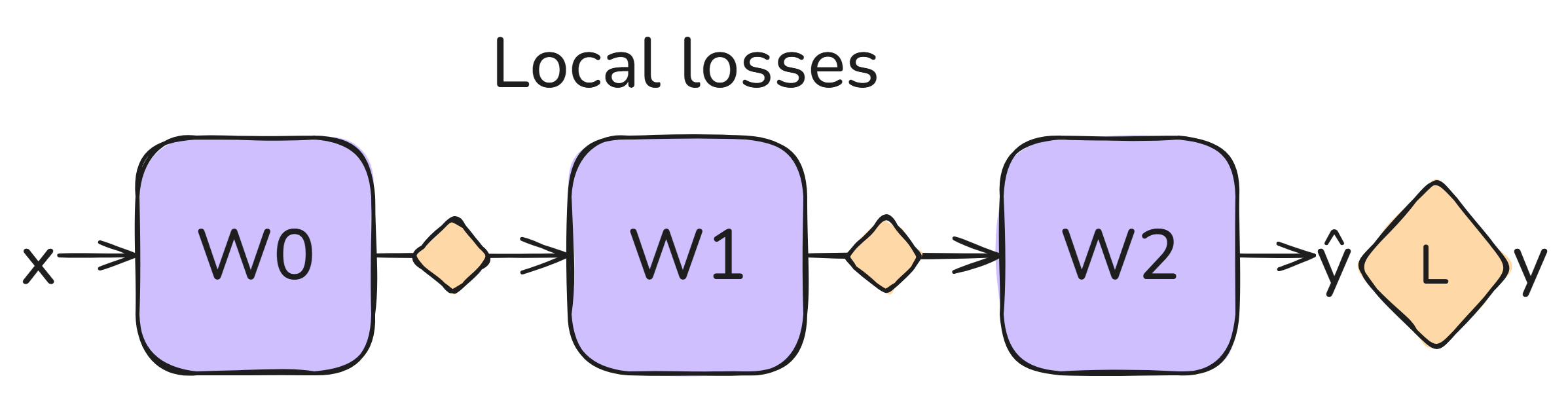
Now, instead of perfectly forwarding a layer’s prediction $\mathbf{\hat{s}_i}$, we allow some slack. We introduce a free variable $\mathbf{s_i}$, representing the input of the next layer. The local loss $\mathcal{L}_i$ tries to tie $\mathbf{\hat{s}_i}$ and $\mathbf{s_i}$ together as closely as possible, but they don’t necessarily have to be equal to one another.
During training, PC tries to find the set of states ${\mathbf{s_i}}$ that minimizes the sum of all of these local losses (typically referred to as the energy $E$):
$$\mathcal{L}_{PC} = \sum_i \mathcal{L}_i + \mathcal{L}_{class}$$
(note that the classification loss has simply become the local loss for the top layer)
With that set of optimal states (typically found via gradient descent), you can perform purely local weight updates which are 100% biologically plausible.
Implications
Okay, so PC is just inserting local losses and finding the states that minimize the sum of the local losses. How is this interpretation more useful than variational inference?
Well, glad you asked. Let’s clear up some confusion and list up some direct consequences and ideas:
- Where’s the squared difference I always see in PC? To get standard PC, just use MSELoss for $\mathcal{L}_i$. If you want to add precision weights, go for Pytorch’s GaussianNLLLoss.
- Can I really use any loss I’d like? Hmmm, not quite. While many losses are secretly negative log likelihoods of some distribution (e.g., MSELoss belongs to a Gaussian), and you can use any distribution you’d like for PC, there are still a few caveats:
- The global loss should be bounded from below. Otherwise, gradient descent will go all the way down to negative infinity! Now, this doesn’t necessarily mean each individual local loss should be bounded, but still, be careful.
- Keep in mind that your target is now $\mathbf{s_i}$, which is variable. This can be a problem for losses that expect the target to have a certain form (e.g., CrossEntropy expects a one-hot).
- You need to account for the distribution’s normalization constant to get correct weight regularization.
- Do other losses lead to other models? Yes! For example, you can get the Continuous Hopfield network from Bengio by using the loss $\mathcal{L}_i = \frac{1}{2} ||\mathbf{s_i}||^2 - \rho(\mathbf{s_i})^T \cdot \mathbf{\hat{s}_i}$.
- Can I use a trainable loss? If you take into account the caveats above, yes you can! For example, you could use a 2D normalizing flow as a componentwise loss. However, the caveats are not always easy to enforce, so you’d have to engineer your way around them.
- Why are local losses enough for global learning? Turns out there’s no need for backprop’s global loss, just some time to spread the information across the local losses. Once that’s done, every layer has its own loss to minimize, as if we had a bunch of parallel 1-layer networks trying to predict a fixed target. I find this pretty remarkable, to be honest!
- Which one is greater: the PC energy or the backprop loss? With standard initialization (which amounts to setting all
$\mathcal{L}_i = 0$), the PC energy at the start will be exactly equal to the backprop loss. Next, we do energy minimization, so we can say that the energy will always be lower than the loss. Probably, the ratio$E/\mathcal{L}_{class}$can be interpreted as something interesting, but I’m not sure what exactly. - How should I implement PC? If you’re not planning on doing anything too fancy, inserting local losses is enough! Most DL frameworks were designed to minimize losses, so it shouldn’t be too much of a hassle. The core of my implementation consists of only around 200 lines.
Going beyond local losses: minimal-norm perturbations
The view of PC as local losses corresponds to the established form of PC doing state updates on free variables $\mathbf{s_i}$. However, in my latest paper, I show that you can go much faster (100-1000x) by directly modelling the errors $\mathbf{e_i}$ instead of the states.
Technical details aside, how can you interpret this in the local loss framework?
Instead of separating $\mathbf{\hat{s_i}}$ and $\mathbf{s_i}$, we simply add a skip connection and define $\mathbf{s_i} := \mathbf{\hat{s_i}} + \mathbf{e_i}$. The standard MSELoss now simplifies to an L2 norm on the errors $||\mathbf{e_i}||^2$. But feel free to choose any other norm!
Instead of local losses, we now have local perturbations that we add to the network predictions.

The goal is to minimize the classification loss while keeping the errors as small as possible (minimal norm):
$$\mathcal{L}_{PC} = \sum_i \|\mathbf{e_i}\|^2 + \mathcal{L}_{class}$$
It’s a bit similar to an adversarial attack, except that you’re now trying to improve the loss instead of degrade it.
You still prefer the local losses? That’s alright. The errors can also be used to speed up the local loss formulation of PC. Just use the definition $\mathbf{s_i} := \mathbf{\hat{s_i}} + \mathbf{e_i}$ and plug it into your favorite loss function.
Outro
No more need for fancy maths: Predictive Coding is just backprop with local losses. I hope this view can help you forward in getting some intuition on PC. Of course, once you get further into the field, it can be very useful to explore the mathematical structure of PC’s graphical networks and its relation to ELBO. But for just a quick introduction? Local losses all the way.